Implementation Notes: Runtime Environment Map Filtering for Image Based Lighting

In this post I will cover implementing and optimizing runtime environment map filtering for image based lighting (IBL). Before we get started, this approach is covered in depth in Real Shading in Unreal Engine 4 and Moving Frostbite to Physically Based Rendering, you should really check them out if you want more background and information than I provide here. Doing runtime filtering of environment maps has some benefits over offline filtered maps (using something like cubemapgen). One is that you can have more dynamic elements in your cubemaps like dynamic weather and time of day. At GDC this year Steve McAuley mentioned in Rendering the World of Far Cry 4 that they perform environment map re-lighting and composite a dynamic sky box prior to filtering. Additionally by filtering at runtime you might be able to use smaller textures (r10g11b10 vs r16b16g16a16) since you can use your current camera exposure information to pre-expose the contents into a more suitable range.

Overview

---

Image Based Lighting involves using the contents of an image (in this case an enviornment map) as a source of light. In the brute force implementation every pixel is considered a light source and is evaluated using a bidirectional reflectance distribution function (BRDF). The full integral that represents this is:

Numerical integration of environment lighting

The variant of filtering that we will be implementing is the Split-sum approach taken by Karis. This approach approximates the integral above by integrating the lighting contribution and the rest of the BRDF separately. By doing this the integral can be approximated using a cubemap and a tex2D lookup.

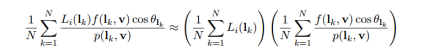
Split-sum approximation

Initial implementation

---

We will start with the implementation provided in Real Shading in Unreal 4 since it is well documented and complete, I will be referring to this as the reference implementation. To assist in reducing the number of samples the authors of the mentioned papers utilized importance sampling to redistribute the samples into the important parts of the BRDF. Importance sampling is a very interesting topic so if you want to learn more about the derivation check out Notes on importance sampling. For the BRDF integration we can stop with this implementation since this won’t be integrated every frame. Also, I’m choosing to ignore the extensions that the frostbite guys did to add the Disney Diffuse BRDF term into this texture but this can apply to that too. The environment map filtering is where we want to focus our optimization efforts.

The first step is to render out a new cubemap to filter. For comparison purposes this article uses the cubemap from the unreal presentation, found here. However; this is the point where you could do some cool stuff like re-lighting the environment map like the Far Cry guys do. As a note, some people use a geometry shader here to render to all faces of a cube in a single pass, for this example I just set up the camera for the appropriate face and rendered them out one at a time.

Foreach Face in Cube Faces
   Setup camera
   Render envmap

Next we implement the split-sum reference implementation provided by Karis. Initially the sample count is kept as provided in the course notes but that is going to be an area we focus on when we optimize.

float fTotalWeight = 0.0f;
const uint iNumSamples = 1024;
for (uint i = 0; i < iNumSamples; i++)
{
    float2 vXi = Hammersley(i, iNumSamples);

    float3 vHalf = ImportanceSampleGGX(vXi, fRoughness, vNormal);
    float3 vLight = 2.0f * dot(vView, vHalf) * vHalf - vView;

    float fNdotL = saturate(dot(vNormal, vLight));
    if (fNdotL > 0.0f)
    {
        vPrefilteredColor += EnvironmentCubemapTexture.SampleLevel(LinearSamplerWrap, vLight, 0.0f).rgb * fNdotL;
        fTotalWeight += fNdotL;
    }
}
return vPrefilteredColor / fTotalWeight;

The code side looks something like this.

Foreach Face in Cube Faces
    Setup camera
    Bind Envmap
    For i = 0; i < MipLevels; ++i
        Set roughness for shader
        Execute filtering

To verify that I didn’t screw anything up I like to reproduce and compare at least one of the diagrams.

Comparison with course notes from Real Shading in Unreal Engine 4.

There is some slight darkening along the rim of the middle gloss spheres due to my angle of view being slightly off, a difference in exposure, and a different tonemapping operator is used but otherwise we are at a good starting point.

Areas for optimization

---

I’m not as crazy as some people when it comes to optimization but here are some questions I ask myself when I’m looking at a bit of code like this.

• What can be done to reduce the amount of work done globally?
• What can be done to reduce the number of samples?
• What can be done to reduce the amount of work per sample?
• How can use any assumptions to our advantage?
• How can we make sure that we are getting the most out of every sample?
• What parts of this can scale?

Luckily the Frostbite guys have already looked into a few of the points above so we can pull from the implementation they provide.

Reduce the amount of work done globally

This one is easy and basically just a footnote in the Moving Frostbite to pbr. Since the first mip is essentially our mirror reflection we can just skip processing that mip level all together and just copy the generated environment map into it. Note that we still keep the generated texture around and copy into our final texture, this becomes more important in the next step. The code now looks like:

Foreach Face in Cube Faces
    Setup camera
    Bind Envmap
    Copy face into mip 0
    For i = 1; i < MipLevels; ++i
        Set roughness for shader
        Execute filtering

Reduce the number of samples

So 1024 samples is certainly more than we want to be doing per pixel in our shader. I would say that 16-32 is a more reasonable number of samples to take. Let’s see what happens if we just drop the number of samples in our shader:

32 Samples

It’s obvious as the roughness increases that 32 samples isn’t going to be enough with out some help. This is where filtered importance sampling comes into play. I’m not an expert on Importance Sampling in general but it was pretty easy to follow along with FIS implementations in the Frostbite course notes. The basic idea is that, because of importance sampling, less samples are taken in certain directions due to the distribution of the brdf. To combat the undersampling the mip chain of the source environment map is sampled. The mip is determined by the ratio between the solid angle that the sample represents (OmegaS) and the solid angle that a single texel is at our highest resolution (OmegaP) covers. Implementing this in the example means that the environment map generation gets the second step of generating mips, additionally for each sample we have to compute OmegaS and OmegaP then finally the required mip.

Foreach Face in Cube Faces
   Setup camera
   Render envmap

GenerateMips envmap

float fTotalWeight = 0.0f;
const uint iNumSamples = 32;
for (uint i = 0; i < iNumSamples; i++)
{
    float2 vXi = Hammersley(i, iNumSamples);

    float3 vHalf = ImportanceSampleGGX(vXi, fRoughness, vNormal);
    float3 vLight = 2.0f * dot(vView, vHalf) * vHalf - vView;

    float fNdotL = saturate(dot(vNormal, vLight));
    if (fNdotL > 0.0f)
    {
        // Vectors to evaluate pdf
        float fNdotH = saturate(dot(vNormal, vHalf));
        float fVdotH = saturate(dot(vView, vHalf));

        // Probability Distribution Function
        float fPdf = D_GGX(fNdotH) * fNdotH / (4.0f * fVdotH);

        // Solid angle represented by this sample
        float fOmegaS = 1.0 / (iNumSamples * fPdf);

        // Solid angle covered by 1 pixel with 6 faces that are EnvMapSize X EnvMapSize
        float fOmegaP = 4.0 * fPI / (6.0 * EnvMapSize * EnvMapSize);
        // Original paper suggest biasing the mip to improve the results
        float fMipBias = 1.0f;
        float fMipLevel = max(0.5 * log2(fOmegaS / fOmegaP) + fMipBias, 0.0f);
        vPrefilteredColor += EnvironmentCubemapTexture.SampleLevel(LinearSamplerWrap, vLight, fMipLevel).rgb * fNdotL;
        fTotalWeight += fNdotL;
    }
}
return vPrefilteredColor / fTotalWeight;

This gives us a much better result for our high roughness spheres, although it is still a little chunky.

32 Samples With Filtered Importance Sampling

Precompute as much as possible

The previous change had the unfortunate side effect of adding lots of math to the inner loop. So lets focus the attention there and see if anything can be pre-computed. First, it should be easy to see that we don’t need to be computing the Hammersley sequence for every single texel in the output, they are the same for every pixel. With this knowledge let’s see how the sequence random value is used:

float3 vHalf = ImportanceSampleGGX(vXi, fRoughness, vNormal);

...

float3 ImportanceSampleGGX(float2 vXi, float fRoughness, float3 vNoral)
{
    // Compute the local half vector
    float fA = fRoughness * fRoughness;
    float fPhi = 2.0f * fPI * vXi.x;
    float fCosTheta = sqrt((1.0f - vXi.y) / (1.0f + (fA*fA - 1.0f) * vXi.y));
    float fSinTheta = sqrt(1.0f - fCosTheta * fCosTheta);
    float3 vHalf;
    vHalf.x = fSinTheta * cos(fPhi);
    vHalf.y = fSinTheta * sin(fPhi);
    vHalf.z = fCosTheta;

    // Compute a tangent frame and rotate the half vector to world space
    float3 vUp = abs(vNormal.z) < 0.999f ? float3(0.0f, 0.0f, 1.0f) : float3(1.0f, 0.0f, 0.0f);
    float3 vTangentX = normalize(cross(vUp, vNormal));
    float3 vTangentY = cross(vNormal, vTangentX);
    // Tangent to world space
    return vTangentX * vHalf.x + vTangentY * vHalf.y + vNormal * vHalf.z;
}

This function can be broken up into two distinct parts shown colored. The first part computes a local space half vector based off the sampling function and the roughness. The second part generates a tangent frame for the normal and rotates the half vector into it that frame. Since the first part is a function of the random value (from the hammersley sequence) and the roughness the local space sample directions can be precomputed. It should also be clear now that we are wasting lots of cycles recomputing the tangent frame for every sample. So we can float that outside of the update loop and just to be complete we can put it into a matrix and rotate the incoming local space sample directions into world space (in reality the shader compiler also noticed this and optimized the math out of the loop).

// Compute a matrix to rotate the samples
float3 vTangentY = abs(vNormal.z) < 0.999f ? float3(0.0f, 0.0f, 1.0f) : float3(1.0f, 0.0f, 0.0f);
float3 vTangentX = normalize(cross(vTangentY, vNormal));
vTangentY = cross(vNormal, vTangentX);

float3x3 mTangentToWorld = float3x3(
    vTangentX,
    vTangentY,
    vNormal );

for (int i = 0; i < NumSamples; i++)
{
    float3 vHalf = mul(vSampleDirections[i], mTangentToWorld);
    float3 vLight = 2.0f * dot(vView, vHalf) * vHalf - vView;
    ....

The next bit of code in the shader reflects the view vector around the half vector to determine the representative light direction for the sample. Following the isotropic assumption made in the split-sum technique we can state that view == normal, and further that in local space normal == 0,0,1. So what we can do here is reflect the vector in local space and instead of rotating the half vector to world space, we can rotate the light vector into world space. There is a problem though, later in the code it assumes that we have the dot product of the half vector and the normal vector to compute the mip-level for the sample. We can once again take advantage of the isotropic assumption and realize that the dot product between two vectors in local space is the same as the dot product of those two vectors in some other space. So ndoth = vdoth = dot((0,0,1),half) or ndoth = vdoth = half.z, therefore this can be precompute per sample now too. Inspecting the code again we see that the mip selection math is based entirely on global variables and those two per sample values, so we can pre-compute that too (see a trend?). Moving all of that computation to the cpu and simply uploading it to the shader leaves us with this:

float fTotalWeight = 0.0f;
const uint iNumSamples = 32;
for (uint i = 0; i < iNumSamples; i++)
{
    float3 vLight = mul(vSampleDirections[i], mTangentToWorld);

    float fNdotL = saturate(dot(vNormal, vLight));
    if (fNdotL > 0.0f)
    {
        vPrefilteredColor += EnvironmentCubemapTexture.SampleLevel(LinearSamplerWrap, vLight, fSampleMipLevels[i]).rgb * fNdotL;
         fTotalWeight += fNdotL;
    }
}

We are back to having less math per sample than before we added FIS and we can still do better. There is still the dot product with the light vector sitting there and the conditional. Once again leverage that we have pre-computed the light vector in local space and say that ndotl = dot((0,0,1), light) = light.z. Additionally, we can check if the weight of a sample is going to be 0 before we even upload it, this lets us just skip samples entirely that will fail the check. At this point the inner loop just rotates the the local light vector into world space and does a madd to accumulate the sample.

for (uint i = 0; i < iNumSamples; i++)
{ 
    float3 vLight = mul(vSampleDirections[i], mTangentToWorld);
    vPrefilteredColor += EnvironmentCubemapTexture.SampleLevel(LinearSamplerWrap, vLight, fSampleMipLevels[i]).rgb * fSampleWeights[i];
}

return vPrefilteredColor * fInvTotalWeight;

Comparison between original and the final optimized version.

Here are some timings for the various approaches and stages of optimizing presented, take them with a grain of salt since getting numbers on PC, especially laptops, is not super accurate.

Device	Time(ms)	Size	Approach
Iris 6100	54.0	256×256	1024 Samples Reference (UE4)
Iris 6100	2.6	256×256	32 Samples FIS Original (Frostbite)
Iris 6100	1.5	256×256	32 Samples FIS Optimized
Iris 6100	1.2	256×256	Varying Sample Count
Iris 6100	0.5	128×128	Varying Sample Count
GTX 980	9.4	256×256	1024 Samples Reference (UE4)
GTX 980	0.48	256×256	32 Samples FIS Original (Frostbite)
GTX 980	0.36	256×256	32 Samples FIS Optimized
GTX 980	0.36	256×256	Varying Sample Count
GTX 980	0.16	128×128	Varying Sample Count

Improvements

---

 Ensure certain number of samples have weight > 0

At high roughness values nearly half of the samples produced by the Hammersley sequence result in a light vector that fails the N dot L check. I noticed a nice improvement by just doing a simple linear search to find how many sequence numbers are needed to generate the right number of valid samples.

Comparison of 32 samples where some have weight 0 (top) and 32 samples where all of them have a weight > 0 (bottom)

Varying the sample count per mip level

This is more or less an extension of the Frostbite statement that the first mip should represent a mirror reflection and therefore require only one sample. If we extend that to the entire mip chain we can simultaneously reduce the number of samples at low roughness values (when we are processing larger cube faces) and increase the number of samples at high roughness values (when the faces are smaller). In theory this will reduce the number of samples needed and result in an overall noise reduction.

Varying sample count on a 256×256 prefiltered cubemap. From mip 0->5: 1, 8, 32, 64, 128, 128

This did result in a nice quality improvement, and dropped the total number of samples taken from the environment map from ~400k to ~200k but I didn’t notice a large performance increase, in fact in some cases I saw the opposite. This is likely due to the small number of pixels requiring lots of work as you get down the mip chain and that increasing the sample count reduces the effectiveness of filtered importance sampling. This approach is still worth investigating though and may be bound by the fact that I render each face individually.

Primary direction lookup

This is straight from the frostbite presentation (See the course notes for details). Basically you modify the reflection vector based on the roughness when retrieving the values from both the environment map and the brdf texture. This makes it look quite different from the initial implementation but if we look back at the Unreal course notes we can see that it looks more like the full reference implementation:

Comparison between the Initial Reference for this article (top), the Reflection Adjusment proposed by the Frostbite team (middle), and the Original Reference in the Real Shading course notes (bottom).

float3 vReflection = 2.0f * vNormal * dot(vViewDirection, vNormal) - vViewDirection;
float fA = fRoughness * fRoughness;
vReflection = lerp(vNormal, vReflection, (1.0f - fA) * (sqrt(1.0f - fA) + fA));

Ideas

---

These are things that I haven’t really fleshed out yet but could potentially be a thing.

Different distribution for filtering

Up to this point we have been using the GGX distribution for the importance sampling but the we are weighting the samples by their respective N dot L terms. This leads to the workarounds in the improvement section to ignore samples that were going to fail the second tier of weighting. It seems that a new probablity distribution could be created that factors in the N dot L weighting so we don’t have to modify and renormalize the distribution later. I briefly fooled around with finding the analytical version of that distribution but I’m not a mathematica guy and ran out of time. Only after did I realize that you could do this with out having an analytical probability distribution function, and instead you can just numerically integration for a fixed roughness value and a set of psuedo-random variables. I plan on investigating this soon.

Different quasi-random sampling set

After doing some research it became apparent that the Hammersley set doesn’t do the best job when you have low sample counts. An alternative sequence may yield lower noise for the same number of samples, here is a potential one that Pixar recently published: Correlated Multi-Jittered Sampling. I tried this out and the results didn’t look exceptionally different, the one thing that did stand out is that you can pass a seed value in to generate any number of 32 sample sequences which might be good if you want to do any sort of progressive filtering of the environment map.

Progressive filtering

Since you know the total weights in the frame it would be easy to pass that data forward to the next frame and combine the results. To do this with the Hammersley sequence you would want to add a rotation into the matrix that rotates the light from local to world space, then you would just filter as usual and add the total weight and result times the total weight from the previous frame. When it comes time to invalidate the environment map you can just start clear the total weight. This may help wrangle the last bit of performance needed for previous gen platforms. Additionally you can track when you get a certain total weight and stop processing all together until you know that the contents have changed, for instance the time of day progresses past a certain threshold.

Conclusion

Hopefully this article was useful to someone out there. It would be great to hear from people if they do other things to optimize this process or have tried any of the things that I proposed.

Resources

---

Light probe used in this article from http://gl.ict.usc.edu/Data/HighResProbes/

Correlated Multi-Jittered Sampling: http://graphics.pixar.com/library/MultiJitteredSampling/paper.pdf

Hammersley Points on the Hemisphere: http://holger.dammertz.org/stuff/notes_HammersleyOnHemisphere.html

Real Shading in Unreal Engine 4: http://blog.selfshadow.com/publications/s2013-shading-course/karis/s2013_pbs_epic_notes_v2.pdf

Moving Frostbite To PBR: http://www.frostbite.com/2014/11/moving-frostbite-to-pbr/

Notes on Important Sampling: http://blog.tobias-franke.eu/2014/03/30/notes_on_importance_sampling.html

GPU Based Importance Sampling: http://http.developer.nvidia.com/GPUGems3/gpugems3_ch20.html

Rendering the world of Far Cry 4: http://www.gdcvault.com/play/1022235/Rendering-the-World-of-Far

Physically Based Shading at Disney: https://disney-animation.s3.amazonaws.com/library/s2012_pbs_disney_brdf_notes_v2.pdf