Implementing a Physically Based Camera

Understanding Exposure
Manual Exposure

The first post in the series described the three key properties of exposure: Aperture (N), Shutter Speed (t), and ISO (S). In this post we will implement manual exposure, meaning that all 3 values are provided by the application or user. Once again this series of posts is heavily inspired by “Moving Frostbite to Physically Based Rendering” ¹ where they cover almost everything presented here in the course notes.

From camera settings to pixel value

To convert from the provided camera settings to a final pixel value we need to know two things: The photometric exposure (H) (amount of light reaching the sensor) and the ISO rating that results in a well exposed image. The photometric exposure is a function of the incoming scene luminance (L), the optics in the lens, the aperture of the lens, and the time that the sensor is exposed to to the light.

$H = \frac{q \times L \times t}{N^2}$

q represents the properties of lens optics and is defined as follows:

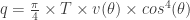
$q = \frac{\pi}{4} \times T \times v(\theta) \times cos^4(\theta)$

Where T is the transmission of the lens (the percent of light that is not absorbed by the optics in the lens), v is the vignetting factor (the characteristic of light falloff from the center of the image to the edges), and $\theta$ is the angle relative to the axis of the lens. To simplify the following equations we will assume the standard q value of 0.65 ( $T = 0.9, v = 0.98, \theta = 10^{\circ}$ ).

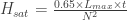
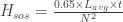
Once the photometric exposure is known the sensors ISO rating can be measured. The ISO standards define five different ways of measuring the ISO rating of a digital sensor. This article will use two of these methods: Saturation-based Speed( $S_{sat}$ ) and Standard Output Sensitivity( $S_{sos}$ ). These methods will be used to solve backwards from a known ISO value (S) to the representative scene luminance and then into an exposure scalar that we can render with.

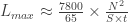
Saturation-based speed

Saturation-based speed rates the ISO using the maximum photometric exposure ( $H_{sat}$ ) that doesn’t lead to pixel values greater than 255/255 (i.e. saturated).

$S_{sat} = \frac{78}{H_{sat}}$

The value 78 was chosen represent an average pixel value of $\frac{18\%}{\sqrt{2}}$ where the $\sqrt{2}$ allows for headroom for highlights². As stated, the saturation-based speed method is solving for the maximum luminance, making the substitution with the photometric exposure we have:

$H_{sat} = \frac{0.65 \times L_{max} \times t}{N^2}$

$S_{sat} = \frac{7800}{65} \times \frac{N^2}{L_{max} \times t}$

Solving for $L_{max}$ :

$L_{max} = \frac{7800}{65} \times \frac{N^2}{S_{sat} \times t}$

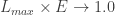
We would solve for an exposure (E) by scaling the luminance such that $L_{max} \times E \rightarrow 1.0$

$E = \frac{1.0}{L_{max}}$

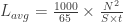
Standard output sensitivity

The standard output sensitivity method is similar the the saturation based method but solves for the exposure that results in pixel values of 118/255 (0.18 encoded with sRGB into an 8-bit pixel).³

$S_{sos} = \frac{10}{H_{sos}}$

Similar to the previous method we will substitute in the photometric exposure but we will solve for $L_{avg}$ instead.

$H_{sos} = \frac{0.65 \times L_{avg} \times t}{N^2}$

$S_{sos} = \frac{1000}{65} \times \frac{N^2}{L_{avg} \times t}$

$L_{avg} = \frac{1000}{65} \times \frac{N^2}{S \times t}$

This time when solving for the exposure we determine what exposure would yield 18% ( $L_{avg} \times E \rightarrow 0.18$ ).

$E = \frac{0.18}{L_{avg}}$

As you can see the two equations are nearly identical in how they measure the ISO speed rating. In fact, if we were to state that $\frac{18\%}{\sqrt{2}}$ should represent the average luminance instead of $18\%$ and we assumed that we were simply applying a gamma curve to a linear input then they are equivalent!

$L_{avg} = 0.127 * L_{max}$

$0.127 * L_{max} = \frac{1000}{65} \times \frac{N^2}{S \times t}$

$L_{max} \approx \frac{7800}{65} \times \frac{N^2}{S \times t}$

Tonemapping Considerations

The intention of these exposures is to end up with a well exposed image (i.e. an average pixel value of 118).18% is chosen because it is assumed that a standard gamma curve is being applied: $\frac{118}{255}^{2.2} = 0.18$ . However; this is not true in most games. Instead we map the scene luminance values using a tonemapping operator (I suggest checking out John Hable’s post if you need some background information). This means that we should modify our exposure calculations to compensate for that. This can be done to both SBS and SOS measurements but it is easier to see how it would integrate with the SOS method.

As the last step of converting the luminance value into an exposure we use 18% as the middle grey value. To adjust for your tonemapping operator we just need to solve for the input value that results in a pixel value of 118/255.

$T(x) = \frac{118}{255}$

We do this by either applying the inverse tonemapping operator (if your tonemapper can be inverted), or use some graphing software to solve for the intersection of $y=\frac{118}{255}$ .

Using the optimized tonemapper by Jim Hejl and Richard Burgess-Dawson ⁴ $x \approx 0.148$ . Substituting this value in to find the exposure we end up with:

$E = \frac{0.148}{L_{avg}}$

These equations are extremely straightforward to implement in code:

/*
* Get an exposure using the Saturation-based Speed method.
*/
float getSaturationBasedExposure(float aperture,
                                 float shutterSpeed,
                                 float iso)
{
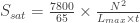
    float l_max = (7800.0f / 65.0f) * Sqr(aperture) / (iso * shutterSpeed);
    return 1.0f / l_max;
}

/*
* Get an exposure using the Standard Output Sensitivity method.
* Accepts an additional parameter of the target middle grey.
*/
float getStandardOutputBasedExposure(float aperture,
                                     float shutterSpeed,
                                     float iso,
                                     float middleGrey = 0.18f)
{
    float l_avg = (1000.0f / 65.0f) * Sqr(aperture) / (iso * shutterSpeed);
    return middleGrey / l_avg;
}

Validating the results

We haven’t talked about converting lighting units to photometric units yet (but we will) so to validate that we have decent exposure settings we will turn to the Sunny 16⁵ rule. This rule states that when the aperture is set to f/16.0 and the shutter speed equals the inverse of the ISO we should have a good exposure for a typical sunny day. From tabular data we find that the expected EV for a sunny day respecting this rule would be around 15. Again from tabular data a standard lightmeter reading of 15 EVs would represent an average luminance of $\approx 4096$ .⁶ Substituting into:

$L_{avg} = \frac{1000}{65} \times \frac{N^2}{S \times t}$

$L_{avg} = \frac{1000}{65} \times \frac{16^2}{100 \times \frac{1}{100}}$

$L_{avg} \approx {3938}$

This value is very close to what we would expect to expose for so we are in the ball park. And here is a test scene exposed using the Sunny 16 rule. The average scene luminance is $\approx 4000$ and we end up with a well exposed image.

In the next post in the series we will cover the various methods for implementing automatic exposure.

Steve beat me to it. This is essentially the conclusion we reached for tonemapping on AC Unity: let the tone curve handle this.

Originally we used a tweaked version of the Uncharted 2 tone curve (drawing from Joshua Pines’ presentation) but later switched to using a log s-curve from the appropriate ACES ODT, which compresses a few more stops at the high end (which reduced ‘burning’ in extreme sunlight situations). I believe it’s also a touch less contrasted in the darks, which was desirable since we applied grading on top of this (we also wanted a ‘neutral’ view for material evaluation).

We also started out by doing SOS, but moved to the saturation approach when we switched to using *diffuse lighting* for adaptation — essentially what Kojima Productions were advocating at GDC’13 (I think Naty also made a similar suggestion in his keynote at I3D’13).

Regarding manual exposure, I started out using the same formulas (first two equations) as well, and I remember even going further taking measurements with a camera. However, in the end, this was a bit of a pointless exercise; it’s a lot easier to just use the standard formulas that relate camera settings to EV and EV to luminance (L):

EV = log2(fNumber*fNumber/shutterTime)*100/iso)

EV = log2(L*100/K)

… using the standard calibration constant (K = 12.5, for typical DSLRs and spot meters).

Working with EV was convenient, as it was easy for artists to get their heads around. As a result we used EV as an input option for lights, displayed a debug luminance grid in EV and used an EV bias curve (really a table) in order to to counterbalance autoexposure in low-light conditions.

I’d been meaning to write this up in more detail, but that’s the gist for now. 🙂

LikeLike

8 thoughts on “Implementing a Physically Based Camera: Manual Exposure”

Steve McAuley (@stevemcauley) on November 21, 2014 at 2:54 pm said:

Nice article Padraic! However, I’m not sure that we need to take tonemapping into account. For example, ACES assumes that an 18% grey card maps to 0.18 in scene-linear space, which then has tone mapping applied to that image. In fact I think it maps 0.18 in scene-linear to 0.10 in display-linear, which is what Joshua Pines mentioned in his talk at Naty Hoffman’s colour course at SIGGRAPH 2010. Hence I believe we should be aiming to achieve an average luminance of 0.18 in scene-linear space, then be content to let our tone mapping pipeline take charge after that.

LikeLike

Reply ↓
- padraichennessy on November 21, 2014 at 3:19 pm said:
  
  That is good insight. The literature seemed to prioritize the output value over the scene linear. On page 20 of http://www.cipa.jp/std/documents/e/DC-004_EN.pdf they state that the Standard Output Sensitivity relates to a final pixel value of 118. But I have seen it referenced both ways.
  
  LikeLike
  
  Reply ↓
  - Stephen Hill (@self_shadow) on November 24, 2014 at 12:12 am said:
    
    Steve beat me to it. This is essentially the conclusion we reached for tonemapping on AC Unity: let the tone curve handle this.
    
    Originally we used a tweaked version of the Uncharted 2 tone curve (drawing from Joshua Pines’ presentation) but later switched to using a log s-curve from the appropriate ACES ODT, which compresses a few more stops at the high end (which reduced ‘burning’ in extreme sunlight situations). I believe it’s also a touch less contrasted in the darks, which was desirable since we applied grading on top of this (we also wanted a ‘neutral’ view for material evaluation).
    
    We also started out by doing SOS, but moved to the saturation approach when we switched to using *diffuse lighting* for adaptation — essentially what Kojima Productions were advocating at GDC’13 (I think Naty also made a similar suggestion in his keynote at I3D’13).
    
    Regarding manual exposure, I started out using the same formulas (first two equations) as well, and I remember even going further taking measurements with a camera. However, in the end, this was a bit of a pointless exercise; it’s a lot easier to just use the standard formulas that relate camera settings to EV and EV to luminance (L):
    
    EV = log2(fNumber*fNumber/shutterTime)*100/iso)
    
    EV = log2(L*100/K)
    
    … using the standard calibration constant (K = 12.5, for typical DSLRs and spot meters).
    
    Working with EV was convenient, as it was easy for artists to get their heads around. As a result we used EV as an input option for lights, displayed a debug luminance grid in EV and used an EV bias curve (really a table) in order to to counterbalance autoexposure in low-light conditions.
    
    I’d been meaning to write this up in more detail, but that’s the gist for now. 🙂
    
    LikeLike
Pingback: Readings on Physically Based Rendering | Interplay of Light
Pingback: Implementing a Physically Based Camera: Automatic Exposure | Placeholder Art
neoragex2002 on October 29, 2015 at 5:55 am said:

I am so curious about the screen-shot and its lighting. Would you kindly enough to give some suggestions about how to setup the ‘ Sunny 16’-alike light? Thank you!

LikeLike

Reply ↓
- Padraic Hennessy (@padraichennessy) on October 29, 2015 at 6:50 pm said:
  
  sure! I actually have spent a fair bit of time noodling around with a solid ambient model. I started by just getting the ratio of lighting to be correct, for this I looked at some older literature for architecture to get a simple mathematical representation. I validated the results with light meter readings that are referenced in a couple papers like the frostbite one. Then I got the sun set up in a similar fashion by applying a scattering model to get the right intensity, once again validating against light meter readings. I was hooked on skies and lighting for a little bit so I replaced the luminance only representation with the preetham sky model and did a bunch of samples to get a single value for ambient. Then I changed that to spherical harmonics and projected the lighting into that to get a directional ambient term. Finally I wanted to address the issue of specular from the ambient so I did some work on pre-filtering environment maps (see my latest post). I just render the skybox into that cubemap and then pre-filter for the ambient contribution. The sun stayed pretty much the same but I might address that next.
  
  LikeLike
  
  Reply ↓
C0dR on November 17, 2015 at 8:25 pm said:

I am currently working on a physically based camera model for my bachelor and came across your blog. So I tried to implement it myself in OpenGL. I thought of calculating the exposure using the function getSaturationBasedExposure and pass that value to a shader where I will multiply the final color with that value:

colorOut = color * exposure;

But the values I get from that function are way too small (like around 0.00025 etc) so I guess I am missunderstanding the returned value of that function. In your test scene you mention that the scene luminance is around 4000, but I haven’t seen a shader implementation working with color range from 0 to 4000+ (not even HDR goes that high, right?).

So could you explain me how to apply the calculations correctly to a OpenGL scene or help me understand the meaning behind the calculations or maybe even send me the source code of your implementation?

LikeLike

Reply ↓